Basic HTML Version


107
IBRACON Structures and Materials Journal • 2013 • vol. 6 • nº 1
L. A. F. de Souza | R. D. Machado
Where
E
ci
=
E
c0i
(1-
D
ji
), with
j
=
C
,
T
, is the damaged concrete longi-
tudinal elasticity module of the i-th layer. In this example, the cross-
section of the beam was divided into 60 equal layers. The second
portion refers to the equivalent bending stiffness for the steel
EI
eqa
and it is determined by the following expression:
(33)
EI
eqa
=Σ
k=1
nb
E
ak
(
(
π
Ø
k
4
64
+
π
Ø
k
2
4
y
ai
2
Where
n
b
is the number of bars;
φ
k
is the bar diameter
k
;
E
ak
is the
longitudinal modulus of elasticity of the bar steel
k
; and
y
ai
,
i
= 1, 2,
is the distance from the bar centroid
k
to the geometric center of
the cross-section of the beam. Thus, the total equivalent bending
stiffness
EI
eq
is calculated, in a simplified way, by the sum of the
portions
EI
eqc
and
EI
eqa
:
(34)
EI
eq
=EI
eqc
+EI
eqa
When obtaining the vector of the internal elemental force, the
equivalent bending stiffness is determined for each Gauss point in
the numerical integration using the Gaussian Quadrature method.
In the process for calculating the equivalent stiffness, in order to
simplify it, we suppose that the neutral line (
s
x
= 0) is located in the
centroid of the cross-section; this condition is valid if there is a sym-
metry of the armature (lower and upper longitudinal armatures with
the same area and symmetrically positioned in relation to the cen-
troid) and if the materials have a linear elastic behavior (Hooke’s
law). However, when the materials (concrete and/or steel) present
a non-linear behavior, the location of the neutral line is altered.
Thus, in a non-linear analysis, the positioning of the neutral line is
altered for each numerical iteration.
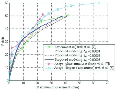
The results obtained from the computational simulations with the
proposed modeling varying the
ε
d0
parameter are shown in Figure
2, as well as the experimental and numerical curves (obtained with
the Ansys software) presented in the work of Jarek
et al
. [7]. This
example shows an important aspect of the Mazars’ model in rela-
tion to the sensitivity of the results with regards to the variation of
the parameter
ε
d0
. The damage determined at the Gauss points
appear in the material when the equivalent strain reaches the ref-
erence strain
ε
d0
, occasioning thus, the stiffness decrease in the
corresponding point.
In accordance with Figure 2, it can be seen that the predicted nu-
merical responses with the proposed modeling for the beam are
more stiff (smaller displacements) for
ε
d0
equal to 0.00003 and
0.00005 up to a given load increment, if compared to the experi-
mental ones. Differently, for
ε
d0
equal to 0.00001, the maximum
displacement
v
takes on higher numerical values from the begin-
ning of the analysis. It can also be noticed that there is a linear
behavior trend in the load-displacement relation from a certain load
value and it maintains itself up to the rupture point. According to
the authors Guello and Bittencourt [5], simulations with the Mazars’
model can lead to excessive strains in the structure from a given
loading. In order to limit these strains, these authors suggest limit-
ing the damage value during the analysis, i.e., have
D
T
< 1 and
D
C
< 1. However, such restrictions were not considered in the simula-
tions carried out with the proposed modeling.
Considering the uniaxial stress case (σ
1≠
0, σ
4≠
0 and σ
2
=0), Equa-
tion (23) is re-written the following way:
(35)
F
1
σ
1
+F
11
σ
1
2
+F
44
σ
4
2
=1
For all the simulations achieved by varying
ε
d0
, the beam collapses
when
P
reaches a value of approximately 50 kN, getting close to
the experimental rupture load. In the computational model, it is
considered that the part fails when one of the finite elements of the
mesh, in one of the Gauss points, fails, i.e., when the inequality
F
1
σ
1
+F
11
σ
1
2
+F
44
σ
4
2
>
1 is satisfied
(result evaluated from the de-
termination of the maximum stresses in the corresponding cross-
section: σ
1
=σ
x
and σ
4
=σ
x
/2
).
Differences in the answers obtained from the three-dimensional mod-
els (with plate and disperse armatures) with the help of the Ansys
software
(Jarek
et al.
[7]) and the implemented in this work. These dif-
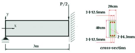
Figure 1 – Structural model of the
beam supported by two points
Figure 2 – Maximum displacement
curve
versus
load increment

